Drafting My Fantasy Football Team With Dynamic Programming

Figure 1: DALLE 3, "Fantasy Football Sisyphus"
Intro
Fantasy Football is a fun game to play with your friends.
For the past four years, I have been developing increasingly complex ways to draft my fantasy football team. I've tried:
- Search (Undocumented)
- Deep Reinforcement Learning
- GPT-4
After spending all this time on algorithms, I've always wondered: how much does the draft actually matter? What is the difference in outcomes between a bad, good and average draft? This year I'll try to both answer this question and write a new drafting algorithm.
Approach
Normally, I like to try to use cutting-edge techniques from machine learning in my algorithm. Unfortunately, machine learning has become a solved problem now and there is nothing new since we covered large language models last year1. Instead, I am going to do a bit of a throwback and use some simple dynamic programming.
The corresponding code for this post is written in haskell. The main thing that
we will be focusing on is the different draft strategies that have been
implemented. A DraftStrategy takes an integer corresponding to the ID for the
team, the current draft state, and returns the player to draft.
type DraftStrategy = Int -> DraftState -> IO Player
The DraftState data type that has information about the current pick, the
available players and the other teams. Perhaps the simplest algorithm that we
can implement with this is just picking a random player.
randomDraftPlayer :: DraftStrategy
randomDraftPlayer teamId state =
  do
    -- Get a list of the avalible players
    let lst = Data.Set.toList (availablePlayers state)
    -- random sample a player from this list
    index <- randomRIO (0, Data.List.length lst - 1)
    return (lst !! index)
I am going to use a lot of the simplifications from the original Deep Reinforcement Learning algorithm2. Instead of trying to select which player to draft out of all of the possible players, we will select the best position out of all of the main offensive positions (QB, RB, WR, TE). This dramatically simplifies the number of potential choices for every draft pick.
For the selected position, we then can just get the player with the highest projected points at that position3. At the level of abstraction we are working at, there is never any value in selecting a player with a lower projected point total for a specific position.
As an additional simplification, we will not consider bench spots. Once a starting line up is filled (9 players) we consider the draft to be over. This means the goal of the draft is simply to fill the initial starting line up (ignoring defenses and kickers).
These assumptions greatly simplify the problem, but I would argue that they maintain the key properties of draft decision making. During a live draft, the main thing that you are thinking about is the relative ordering in which you fill out your team. This ordering mostly matters in the first few picks, with the last few picks mostly reserved for flyers and rookies.
We can now make an improved random algorithm that just selects one of these four highest projected players.
randomGoodPlayer :: DraftStrategy
randomGoodPlayer _ state =
  do
    -- Get the best available players at all positions
    let potentialPlayers = getPotentialBestPlayers teamId state
    -- Randomly select one of those players
    index <- randomRIO (0, Data.List.length potentialPlayers - 1)
    return (best !! index)
An obvious flaw with both of these first two algorithms is that they don't take into account the existing team composition. The above algorithms will have no qualms about drafting 9 quarterbacks in a row, even though we can only put a maximum of two in our starting line up.
We can think of each player's value as how many points they contribute to our the lineup at the end of a draft. If a player fits in the lineup, they contribute their projected points. If they don't fit, they contribute nothing.
In that regard, it will also then never make sense to draft a player that does not fit into our lineup. We can constrain our selection to find players at positions that have corresponding open roster spots. Instead of randomly selecting a position, we can select the best player that we have a spot for. This will nicely fill up our lineup with high scoring players, very similar to what your standard "autodraft" functionality would do. We will refer to this strategy as autodraft.
valuePlayer :: Player -> IO Float
-- Returns the projected points of a player, details aren't important. Reads
-- from a database.

evalPlayers :: (Player -> IO Float) -> Int -> DraftState -> IO [Float]
-- Gets the highest projected point players at each position for a state, and
-- computes their value with the given function.

autoDraftPlayer :: DraftStrategy
autoDraftPlayer teamId state  =
  -- Find the best players that could fill an empty spot on the players team
  let potentialPlayers = getPotentialBestPlayers teamId state
    -- Find the values of these players
    playerValues <- evalPlayers (valuePlayer) teamId state
    -- Find the player with the highest value
    player = getMaxPlayerValue (Data.List.zip potentialPlayers playerValues)
  in case player of
    Nothing -> error "Couldn't find player"
    (Just player) -> return player
In general, we can turn any function that computes the value of drafting a player into a drafting strategy, assuming we always want to select the highest value. Let's define a new type for these kinds of functions.
type PlayerEval = Int -> DraftState -> Player -> IO Float
Then, anything that implements this type can be converted into a drafting strategy as follows.
draftByValue :: PlayerEval -> DraftStrategy
draftByValue evalFn teamId state  =
  let potentialPlayers = getPotentialBestPlayers teamId state

    -- Find the values of these players based on the custom evaluation function
    playerValues <- evalPlayers (evalFn) teamId state

    player = getMaxPlayerValue (Data.List.zip potentialPlayers playerValues)
  in case player of
    Nothing -> error "Couldn't find player"
    (Just player) -> return player

autoDraft :: DraftStrategy
autoDraft = draftByValue (\_ _ x -> valuePlayer x)
Can we improve autodraft? One of the things that makes the fantasy football draft interesting is that different positions score points in very different ways. Quarterbacks generally score the highest, for example. But the gap between the best quarterback and the 5th best quarterback is normally a lot smaller than the gap between the best and the 5th best tight end.
The current algorithm selects the highest projected player at every step. This will not take this dynamic into account at all, and consistently load up on QBs early rounds. Our goal is not to maximize the raw value of any single pick, but the total value of the team at the end of the draft.
However, we can't easily forecast our future team. The available players at the next pick will entirely depend on what our opponents will do. Even with these simplifying assumptions, the complexity of trying to model the full draft is daunting. For the first round alone, there are \(4^12 = 16,777,216\) unique drafts that can occur.
We can make a another simplifying assumption and say that our opponents are going to behave deterministically. This is a poor assumption for real world behavior, but it will give us something of an upper bound for how useful our eventual search algorithm will be.
An okay assumption might be that everyone else will be autodrafting. Although this is a poor model for individual behavior, it likely works well enough in the aggregate. Between any players' picks, the most likely players to come off the board are the highest scoring players at any one position.
What we can now do is try to value a player not by their short-term contribution to the team value, but the long-term value of the final team. To do so, we can rely on the fact that we can now perfectly forecast how the draft will conclude for any given player.
The following haskell function takes a player and the current DraftState and
returns what the final team value for drafting that player will be.
greedyRolloutValue :: PlayerEval
greedyRolloutValue teamId state player =
  do
    -- Apply the pick to the state
    let nextState = stepPlayer teamId player state
    -- Run an AutoDraft simulation to the end
    finalState <- autoDraftSim state
    -- Return the final value of the team
    return (scoreTeam teamId finalState)
We can use this to pick players by simply enumerating our four choices, seeing what the future value would be for each player, and then selecting the player that leads to the highest future team value.
We can reuse the function from before to implement this behavior.
draftGreedysearch :: DraftStrategy
draftGreedysearch = draftByValue (greedyRolloutValue)
We can also use this to value not the selection of a single player (or, action in RL terms), but the pick (or, state) itself. Since we know that we will be selecting the player with the highest greedy rollout value, the value of any one pick is the maximum greedy rollout value from any of the players we could pick within that selection.
greedyRolloutStateValue :: Int -> DraftState -> IO Float
greedyRolloutStateValue teamId state

  -- If the draft is already over, just return the value of the team
  | (isDone state) = return (scoreTeam teamId state)

  -- Otherwise, return the maximum greedy rollout value of the players we could
  -- draft.
  | otherwise = fmap maximum (evalPlayers (greedyRolloutValue) teamId state)
Using this algorithm to pick our players brings up a bit of a contradiction. We select players based on the future team value we would get assuming that we were autodrafting. But by using this criteria we are no longer autodrafting!
To take this into account, let's not try to forecast our own future behavior. Instead, let's think about the relationship between the value of the action of selecting a player and the value of being in the state to pick itself. From our assumptions, we know that:
- The value of a team at the end of the draft is the sum of the projected points of the players in the lineup.
- The value of a state is the maximum of the potential action values within that state.
- The value of the action is the value of the state that results from that action.
We can write these three relationships as two compact functions in haskell.
stateValue :: Int -> DraftState -> IO Float
stateValue teamId state

  -- (#1) If the draft is already over, just return the value of the team
  | (isDone state) = return (scoreTeam teamId state)

  -- (#2) Otherwise, the value is the maximum value of the actions
  | otherwise =
    fmap maximum (evalPlayers stateActionValue teamId state)

stateActionValue :: PlayerEval
stateActionValue teamId state player =
  do
    -- Apply the pick to the state
    let addedPlayerState = stepPlayer teamId player state
    -- Simulate until the next pick for this player
    nextState <- autoDraftSimUntil teamId addedPlayerState
    -- (#3) The value of an action is the value of the resulting state
    stateValue teamId nextState
These few lines will implement a depth first search that will always find the optimal team.
We can see why this is by stepping through the algorithm a bit. We start by trying to find the value of drafting a player. To find the value of drafting that player, we need to find the value of the next state. To find the value of the next state, we need to find the values of the players that we could draft in the next state, and so on. Eventually, we will hit a terminal state that we can value exactly, which will allow us to exactly value the selection of a player, which will allow us to value the preceding state. This will then go all the way back to the original player.
This kind of dynamic programming is at the heart of more traditional reinforcement learning algorithms.
Of course, running this function will always require fully enumerating the
entire tree. To speed things along a bit, we can implement a depth truncated
version that fully enumerates the tree to a given depth, and then uses the
greedyRolloutStateValue to estimate the remaining value of the state.
stateValueDepth :: Int -> Int -> DraftState -> IO Float
stateValueDepth depth teamId state
  | (isDone state) = return (scoreTeam teamId state)

  -- If we've hit our max depth, just value based on a greedy rollout
  | (depth == 0) = greedyRolloutStateValue teamId state

  -- Decrement the depth defore searching the next state
  | otherwise =
    fmap maximum (evalPlayers (stateActionValueDepth (depth - 1)) teamId state)

stateActionValueDepth :: Int -> Int -> DraftState -> Player -> IO Float
stateActionValueDepth depth teamId state player =
  do
    let addedPlayerState = stepPlayer teamId player state
    nextState <- autoDraftSimUntil teamId addedPlayerState
    -- Pass depth along to action value
    stateValueDepth depth teamId nextState
This is important in practice since we only have a minute to make our decision during the actual draft.
We can then wrap these into a drafting functions, very similar to those before.
draftSearch :: DraftStrategy
draftSearch = draftByValue stateActionValue

draftSearchDepth :: Int -> DraftStrategy
draftSearchDepth depth = draftByValue (stateActionValueDepth depth)
Analysis
We are going to analyze the difference in performance for the following algorithms:
- AutoDraft: Selects the position with the highest projected points that has a spot available for it on the roster.
- Bad Auto Draft: Lower bound in performance. Acts like autodraft except it picks the position with the lowest project points.
- Greedy: Selects the player with the highest future value using
GreedyRolloutValue - Search: Selects the player with the highest future value using
stateActionValueDepth, using various depths.
For this draft, we will assume there are 12 total players, and we are drafting 4th. If we run autodraft for everyone, we get the following baseline performances.
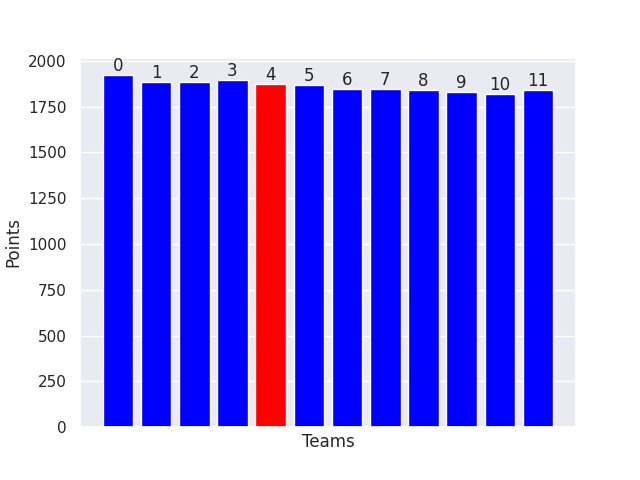
As you might expect, the value of each position decreases from 1st to last. The fourth place position here gets about 1875 points.
We can now run each of our four algorithms to get a feel for the range of performance.
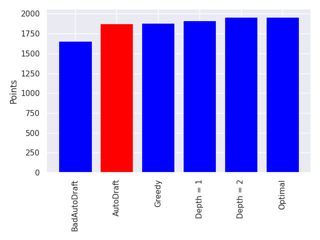
Bad Auto Draft, the approximate worst case, gets 1656 points. The optimal performance is 1961. This gives us a total maximum range of 305 points, or only about 18 points per game.
Everything fit into the expected ordering. AutoDraft is worse than the greedy search, which is worse than the depth limited searches, and so on. Somewhat surprisingly, the maximum performance is also reached doing the truncated depth search at only a depth 2, meaning you really don't need to search that deep.
This is the version that I ended up using when I actually ran the algorithm on draft night, since it comfortably fit within the allowed selection time, giving me leeway to run it again if there was an error.
We can get a feel for how sensitive this performance is by running randomized versions of the AutoDraft strategies. Instead of selecting the highest or the lowest projection, we randomly select the position to draft. We ran this 1000 times against autodraft for the following plot.
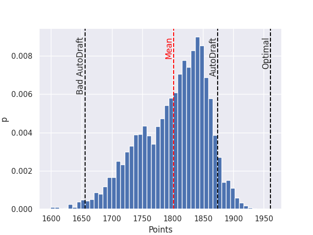
It looks like most of the randomly sampled drafting strategies cluster themselves towards autodraft, but are comfortably worse on average. This plot also highlights the fact the Bad AutoDrafting is not the true lower bound in performance, a small number of the random samples actually ended up performing worse.
Potentially more interesting is the actual drafting strategies that each of these different algorithms end up discovering.
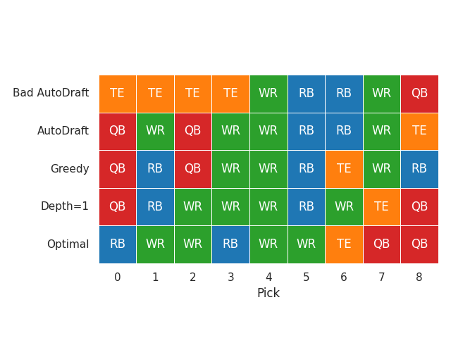
As you might expect, Bad AutoDraft loads up on low scoring TEs. The search algorithms with a more limited horizon take the traditionally high value positions earlier on in the draft. The optimal strategy is particularly unique in that it holds off on drafting any QBs until the final two rounds.
The late QB strategy is very contradictory to human behavior. For a two QB league, most teams will lead with two QBs in the earlier rounds. Potentially, this represents the strategy "overfitting" to the fact that be assuming everyone else is autodrafting we are making this behavior even more extreme.
Conclusion
We can evaluate these strategies in terms of their regret: how many points we lose compared to the optimal strategy every game.
| Algorithm | Regret (Per Game) |
|---|---|
| Bad Auto Draft | 17.9 |
| Random Valid | 9.4 |
| Auto Draft | 5.1 |
| Greedy Search | 4.6 |
| Search (Depth = 1) | 2.6 |
| Search (Depth ≥ 2) | 0 |
| Optimal | 0 |
These numbers are fairly small when you really get into it. AutoDrafting only loses about 5 projected points per game. That is well within noise of the projections themselves. Even simple optimization algorithms can cut this down to less than 4 points per game, equivalent to a single touchdown.
This would heavily imply that the draft itself is not very important. Here we assumed the friendliest assumptions to make the search algorithm as powerful as it could be. Even with these assumptions, we are only gaining five points per game over a strategy of just simply picking the highest value player who can fit on your team.
What does this mean for drafting in practice? Often times people are surprised by how well players who autodraft end up performing. These results would imply that autodrafting is really not a bad strategy at the end of the day. In fact, it is far easier to underperform it than to overperform. The separation between autodrafting and the average random performance is much larger than between autodrafting and the optimal performance. Maybe autodrafting based on high quality estimates is just the way to go?
But how these estimates translate into actual success is another, much more fraught, question. See you next year.