A Big-O for Learning: Thinking with PAC Bounds

First, lets try to define a framework for "machine learning." We have an input space, \(\mathcal{X}\). This is the underlying type that will use to represent the data that will be fed into our model. For example, if \(\mathcal{X} = \mathbb{R}^2\), then our input or raw data is going to be two dimensional real numbers.

We have the output space, \(\mathcal{Y}\). This could be a list of classes, (e.g. \(\mathcal{Y} = \{\text{``cat''}, \text{``dog''} \}\)), or an estimated value for a regression problem (e.g. \(\mathcal{Y} = \mathbb{R}\)). For this installment, we will focus on binary classification problems, \(\mathcal{Y} = \{ 0, 1 \}\), which we will represent as booleans.

What we want to learn is a function, or concept, that maps from the input space to the output space. Mathematically,

In haskell, we can make a type synonym for clarity,

type Concept x y = x -> y

In order to learn this function, will have some dataset, \(S = ((x_1, y_1), \dots, (x_m, y_m))\). Each \(x_i \sim \mathcal{D}\), where \(\mathcal{D}\) is some distribution.

In haskell, we will be using the Control.Monad.Random module for handling random numbers. Again, we can use a type alias to clean things up a bit. We will have our distribution,

type Distribution x = Rand StdGen x

From which we can sample a list of data points,

sampleFrom :: Int -> Distribution x -> Distribution [x]                                         
sampleFrom m dist = sequence (replicate m dist)     

This function takes an integer \(m\) and a distribution and returns m samples from that distribution. Given a list of samples \(\in \mathcal{X}\), we can generate a dataset by simply applying the concept to all of the generated points.

labelData :: Concept x y -> [x] -> [(x, y)]                                                     
labelData concept dataList = map (\x -> (x, concept x)) dataList

In other words, given a concept \(c\) and a list of \(m\) samples \(x_0, x_1, \dots, x_m\) s.t. \(x \in \mathcal{X}\), we can construct a dataset \(S\) as \((x_0, c(x_0)), (x_1, c(x_1)), \dots (x_m, c(x_m))\).

Let's say we have a another concept, \(h\), defined over the same input and output space. More specifically, let's say that \(h\) is the resulting hypothesis of some learning process over data generated by \(c\). How can we evaluate how well it fit the data? Since \(\mathcal{Y}\) is a binary label, we can compute its error with respect \(h\) by measuring the probability that \(h\) and \(c\) disagree over \(\mathcal{D}\),

\(R(h) = 1\) would mean \(h\) and \(c\) never agree while \(R(h) = 0\) would mean that \(h\) and \(c\) always agree. Note, that this doesn't mean that \(h\) and \(c\) are identical, or that \(h(x) = c(x) \forall x \in \mathcal{X}\), just that \(h\) and \(c\) give identical labels to data generated by \(\mathcal{D}\).

Computing \(R(h)\) analytically is difficult, but it is easy to swap it out for an empirical estimate,

We can compute this in haskell as well. First, given a labeled point \((x, y)\), we can check if \(c\) outputs the correct label as,

isIncorrect :: (Eq y) => Concept x y -> (x, y) -> Bool
isIncorrect c (x, y) = (c x) /= y

Then, we can apply this over an entire dataset and compute the portion of incorrectly labeled examples,

errorOf :: (Eq y) => Concept x y -> [(x, y)] -> Float
errorOf concept dataList = 
    let evalList = map (\x -> if isIncorrect concept x then 1.0 else 0.0) dataList
        total = (fromIntegral . length) evalList
     in (sum evalList) / total

By sampling a large enough set of labeled samples, we can use this function to get a high quality estimate of \(R(h)\).

Let's now fully define PAC Learning. Let's say \(h_{S}\) is the hypothesis returned by the learning algorithm after receiving a labeled sample \(S\). We can then define a PAC-learnable concept class as a concept class \(\mathcal{C}\) such that there exists an algorithm \(\mathcal{A}\) and a polynomial function \(p\) such that for any \(\epsilon > 0\) and \(\delta > 0\), for all distributions \(\mathcal{D}\) on \(\mathcal{X}\) and for any target concept \(c \in \mathcal{C}\), the following holds for any sample size \(m \ge p(\frac{1}{\epsilon}, \frac{1}{\delta})\) ¹:

In other words, the probability of the learned hypothesis \(h_S\) from our polynomial time algorithm having an error less than \(\epsilon\) is greater than \(1 - \delta\). Or, \(h_S\) is probably (with probability \(\ge 1 - \delta\)) approximately correct (error less than \(\epsilon\)).

The first thing worth mentioning about this definition is that there are exactly zero constraints on \(\mathcal{D}\) other than it is consistent for our training and testing data. You should be able to concoct whatever tricky distribution you can think of, and the bound should still hold.

The second thing worth noting is that learning is defined against a concept class that is known to the algorithm a priori. This is the most academic assumption made within this framework. Of course, we usually know very little about the class of function that generated the labels for our dataset. Consider this the upper bound of performance on data generated by these concept classes.

In haskell, we can then represent the PAC learning setup as a tuple containing:

1. The distribution we will use to be sample points from \(\mathcal{X}\).
2. A function to sample a hidden concept \(c\)
3. A learning algorithm that takes a dataset \(S\) and returns a concept \(h_S\)
4. The desired error, \(\epsilon\)

type PACTuple x y = (Distribution x, Distribution (Concept x y), [(x, y)] -> Concept x y, Float)

Given one of these tuples and a dataset size \(m\), we can evaluate whether or not the learning algorithm succeeds as,

pacEvaluate :: PACTuple x Bool -> Int -> IO Bool
pacEvaluate (distribution, generateConcept, learnFn, epsilon) m = do
  -- Sample a hidden concept, c
  hiddenConcept <- evalRandIO (generateConcept)
  -- Create a set of training points, S
  trainPoints <- evalRandIO (sampleFrom m distribution)
  -- Create an evaluation set to estimate R(h_S)
  testPoints <- evalRandIO (sampleFrom 10000 distribution)

  let labeledTrainPoints = labelData hiddenConcept trainPoins
      labeledTestPoints = labelData hiddenConcept testPoints
      -- Learn h_S 
      hypothesis = learnFn labeledTrainPoints
      -- Estimate its error
      measuredError = errorOf hypothesis labeledTestPoints
      -- Check whether this error is less than the desired bound
      success = measuredError <= epsilon

  return success

We can then empirically estimate the \(\delta\) for this algorithm by running the above process multiple times and computing the probability of success,

estimateDelta :: PACTuple x Bool -> Int -> Int -> IO Float
estimateDelta pac m n = do
  val <- sequence [pacEvaluate pac m | x <- [1..n]]
  let failures = map (\x -> if x then 0.0 else 1.0) val
  let mean = (sum failures) / (fromIntegral n)
  return mean

Let's now use this framework to answer a very specific question about learning intervals. If we allow our intervals to be of arbitrary dimensions, how does the difficulty of the learning problem scale with the number of dimensions?

Let's make this more concrete. We can start by working through the simplest example, one-dimensional intervals. Our input space is going to be one dimensional real numbers, \(\mathcal{X} = \mathbb{R}\), and our output space will still be binary. An interval will have a lower and upper bound, and it will only return \(c(x) = 1\) if \(x\) is within these bounds. We can represent this kind of function in haskell as,

isInInterval :: Float -> Float -> Float -> Bool
isInInterval lower upper val = (val >= lower) && (val <= upper)

We can randomly construct an interval by sampling a lower and upper bound,

randomBounds :: Distribution (Float, Float)
randomBounds = do
    valOne <- getRandom
    valTwo <- getRandom
    if valOne < valTwo
        then return (valOne, valTwo)
        else return (valTwo, valOne)

And then applying our isInInterval function,

randomInterval :: Distribution (Float -> Bool) 
randomInterval = do
    (lower, upper) <- randomBounds
    return (isInInterval lower upper)

Our initial goal is to develop a PAC-learning algorithm for this concept class.

Let's say we have a dataset \(S\) of labeled points by some hidden interval \(c\). If we construct a new \(h\), there are two types of ways it can be wrong:

1. A false positive: \(h(x) = 1, c(x) = 0\)
2. A false negative: \(h(x) = 0, c(x) = 1\)

An obvious algorithm would be to take the points in \(S\), find the maximum point such that \(c(x) = 1\) and the minimum point such that \(c(x) = 1\) and use those as the bounds of the interval. We can implement this algorithm by first creating a function that only returns the positive examples in our training set, and then one that then uses those positive points to construct the interval.

getPositivePoints :: [(x, Bool)] -> [x]
getPositivePoints = (map fst) . (filter snd)

pointsToInterval :: [Float] -> Concept Float Bool
pointsToInterval [] = \x -> False 
pointsToInterval positive_points = 
        isInInterval (minimum positive_points) (maximum positive_points)

learnInterval :: [(Float, Bool)] -> Concept Float Bool
learnInterval = (pointsToInterval . getPositivePoints)

This intuitive algorithm has the nice property that it cannot generate any false positives. If we think about these two functions as forming sets of \(\mathcal{X}\) where \(f(x) = 1\), then we know that \(h_S \in c\).

In other words, \(h_S\) will always define a slightly smaller interval than \(c\). For each concept \(f\), lets say the parameters of their intervals are \((l_f, u_f)\) where \(l_f\) corresponds to the lower bound of \(f\) and \(u_f\) corresponds to the upper bound of \(f\). The error between \(h\) and \(c\) is the probability that a point falls in the region between the outer bound of \(c\) and the inner bound of \(h\),

Let's imagine two buffer regions, \(r_l\) and \(r_u\). \(r_l\) is the buffer on the lower region such that the probability of a point landing in \(r_l\) is \(\frac{\epsilon}{2}\). In other words, \(r_l = (l_c, z)\) where \(z\) is whatever value it takes so that

\(r_u\) is defined similarly, but for the upper region. Note that this region is independent of our \(h\).

Let's say that \(h_l < r_l\) and \(h_u > r_u\), which means our learned interval intersects with these buffer regions. We then know that,

In other words, if both of the upper and lower bounds of our learned interval \(h\) fall in the buffer regions, we know that the error is less than \(\epsilon\). What is the probability of this happening?

We know that by definition for each buffer region,

That means that for every sample from \(\mathcal{D}\), the probability that the point doesn't fall in \(r\) is \(1 - \frac{\epsilon}{2}\). So the probability that all of our \(m\) points don't fall in the region is,

What is the probability that both don't receive any points? Here, we can greatly simplify the analysis by using a union bound. For any two events \(A\) and \(B\), the probability of both \(A\) and \(B\) occurring is less than the sum of the probabilities of \(A\) and \(B\) individually. Or,

Another fact that will prove useful is that \(1 - x \le \exp(-x)\) for all \(x \in \mathbb{R}\). We can then just say that,

This means that the probability that our learning algorithm will fail to produce a hypothesis with an error \(\le \epsilon\) is \(\le 2 \exp(-m \epsilon / 2)\). Or, in terms of our \(\delta\),

We can then do some algebraic manipulation to show that

This means that for a given error value and desired probability of success, we can definitively say what the lower bound of the feasible dataset size is.

Let's verify this bound by comparing with some empirical data. We can estimate the delta for a series of values of \(m\), and then plot that data. First, we need a function to get this data.

outputData :: PACTuple a Bool -> Int -> Int -> Int -> IO ()
outputData pactuple n step max = do
    -- Create the range of potential m values, the size of the training set
    let mVals = [0,step..max]
    -- For each m, estimate the delta with n samples
    val <- sequence $ [ estimateDelta pactuple m n | m <- mVals]
    -- Format the string for output
    let both = zip val mVals
        fmtString currentString (val, m) = 
                currentString ++ (show m) ++ " " ++ (show val) ++ "\n"
        outputString = foldl fmtString "" both
    putStrLn outputString

We can then create a PACTuple for the interval and generate this data,

let intervalPAC = (getRandom, randomInterval, learnInterval, 0.01) :: PACTuple Float Bool
outputData intervalPAC 300 25 600

Plotting this data, we can see that it does in fact follow the bound.

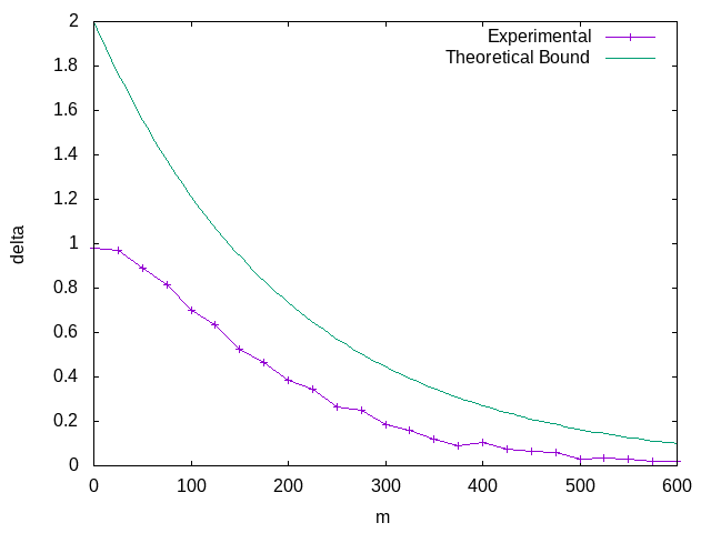
It's worth taking a moment to reflect on what we just were able to prove. We were able to derive a probabilistic bound on the error based on the dataset size alone. Given a \(m\) and \(\epsilon\), you can predict what the probability of success of reaching that \(\epsilon\) is entirely irrespective of the underlying data distribution. Conversely, given an \(\epsilon\) and a \(\delta\), you can determine the \(m\) you need to guarantee you'll satisfy those constraints.

We can generalize the above case to higher dimensions by taking the union of intervals over different dimensions. For example, we can change from an interval to a axis-aligned box in two dimensions by taking the union of two intervals

type Point = (Float, Float)

boxInterval :: Concept Float Bool -> Concept Float Bool -> Concept Point Bool
boxInterval xInterval yInterval = \(x,y) -> ((xInterval x) && (yInterval y))

Our input space here is now \(\mathbb{R}^2\), which we are referring to as the type Point. Our box is defined as an interval in the x dimension and an interval in the y dimension.

We can again randomly sample points and boxes in a very similar method to before,

randomBox :: Distribution (Point -> Bool)
randomBox = do 
    xInterval <- randomInterval
    yInterval <- randomInterval
    return (boxInterval xInterval yInterval)

randomPoint :: Distribution Point
randomPoint = do
    valOne <- getRandom
    valTwo <- getRandom
    return (valOne, valTwo)

And our learning function will require simply splitting up the learning problem into the two dimensions,

pointsToBox :: [Point] -> (Point -> Bool)
pointsToBox [] = \x -> False
pointsToBox positive_points = 
       let xInterval = pointsToInterval (map fst positive_points)
           yInterval = pointsToInterval (map snd positive_points)
        in boxInterval xInterval yInterval

learnBox :: [(Point, Bool)] -> Concept Point Bool
learnBox = (pointsToBox . getPositivePoints)

We can repeat the exact same mechanism of the proof before, but now we have two regions per dimension. If \(d\) is the dimension of the problem, we can adjust each potential error region to have probability \(\frac{\epsilon}{2d}\) to ensure they still sum to \(\epsilon\). Working through the analysis again with this modification, we get

Before, we only cared about the one dimensional line (\(d = 1\)). Now, we have a box with \(d = 2\). We can again generate some empirical data and again confirm that this bound holds.

let boxPAC = (randomPoint, randomBox, learnBox, 0.01) :: PACTuple Point Bool
outputData boxPAC 300 25 1000

Which we can plot again,

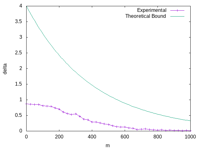
More importantly, we can finally address the question we began with. We can rearrange the above expression to get,

This means that the total sample size required to reach a constant \(\epsilon\) and \(\delta\) is growing \(O(d \log d)\).

The previous proof relies on very specific geometric arguments and learning algorithms. What about something a little bit more general?

Let's think about finite concept classes. These are classes, such as decision trees or programs with an upper limit in bits, which have a finite but usually very large number of possible concepts within the class. These functions can be much more expressive than the simple intervals we introduced in the last section.

In fact, let's not even think about the learning function at all. Let's just assume we have some polynomial time algorithm that will return a concept that is consistent with the \(m\) samples in our dataset. Just based on this alone we can establish a PAC bound.

To see how this works, lets work backwards. For our concept class \(\mathcal{H}\), lets define the set of concepts \(\mathcal{H}_{\epsilon}\) to be the "bad" concepts that have an error greater than \(\epsilon\). Or,

In order to avoid making any assumptions about the algorithm, we can just think about what the probability of any \(h \in \mathcal{H}_{\epsilon}\) being consistent with the \(m\) examples. This is a natural upper bound on the probability of the algorithm returning a hypothesis in \(\mathcal{H}_{\epsilon}\), since it cannot return a bad hypothesis if one does not exist.

What is the probability a bad hypothesis would be consistent with our dataset \(S\)? Since we know \(R_S(h) \ge \epsilon\), we can use a similar argument to the previous proof and say that

But then what is the probability that any of the bad hypothesis will have \(\hat{R_S}(h) = 0\)? Now, we can again use the union bound again to say,

But, we don't really know the size of \(| \mathcal{H}_{\epsilon} |\). However, we do know that \(| \mathcal{H}_{\epsilon} | \le | \mathcal{H} |\) since \(\mathcal{H}_{\epsilon} \subseteq \mathcal{H}\). That then means that,

Or,

We can then solve this expression for \(m\), using some algebraic manipulation

This means the number of samples required is \(O(\log | \mathcal{H} | )\).

Let's work through an example of a finite hypothesis class, conjunctions over \(k\) literals of the form,

Each literal is either:

1. Unused: the value of this literal is ignored
2. Used: the value of this literal is part of the conjunction
3. Negated: the negation of this literal is part of the conjunction

The question we will try to answer is how the problem difficulty is affected by increasing the total number of literals. How much harder is the problem when you have 2 variables versus 16?

We can start our implementation by adding some types,

type BoolVector = [Bool]
type LiteralVector = [Literal]

data Literal = Used | Negated | Unused
             deriving (Eq, Show)

We can then apply each Literal to a bool using,

evalLiteral :: Literal -> Bool -> Bool
evalLiteral Unused _  = True
evalLiteral Negated x = not x
evalLiteral Used x    = x

We can then recursively apply this to a list of bools using,

satisfiesLiteral :: LiteralVector -> BoolVector -> Bool
satisfiesLiteral [] [] = True
satisfiesLiteral l [] = False
satisfiesLiteral [] b = False
satisfiesLiteral (l:otherLiterals) (b:otherBools) = (evalLiteral l b) && satisfiesLiteral otherLiterals otherBools

Generating random literals is a little more complicated than before. First we can write a function that randomly generates literals from a random Float.

floatToLiterval :: Float -> Literal
floatToLiterval val 
  | val <= 0.1 = Used
  | val <= 0.2 = Negated
  | otherwise = Unused

randomLiteral :: Distribution Literal
randomLiteral = do
    val <- getRandom
    return (floatToLiterval val)

The numbers selected in floatToLiteral are arbitrary. We can then use this to sample some random literal expressions to use as our target,

randomLiteralExpression :: Int -> Distribution (Concept BoolVector Bool)
randomLiteralExpression n = do
          random_val <- (sampleFrom n randomLiteral) 
          return (satisfiesLiteral random_val)

We can use the built in getRandom to sample booleans for the BoolVector.

randomBoolVector :: Int -> Distribution BoolVector
randomBoolVector n = sampleFrom n getRandom

Now, we need our learning function. All we need is a function that takes our data and returns a concept that could have potentially generated that data.

We are going to write this is a similar manner to the way we wrote the satisfiesLiteral function. We will first define a local update for every boolean literal pair. We will start by initializing our potential function to be a list of Used literals. For every positive sample in \(S\),

updateLiteral :: Literal -> Bool -> Literal
-- If the Literal is Used and the boolean is True, don't change.
updateLiteral Used True = Used
-- If the Literal is Used and the boolean is False, the concept would have been wrong. Update to Negated.
updateLiteral Used False = Negated
-- If the Literal is Negated and the boolean is True, this literal has been both True and False for a postive sample. Must be Unused.
updateLiteral Negated True = Unused
-- If the Literal is Negated and the boolean is False, don't change.
updateLiteral Negated False = Negated
-- Once marked Unused, it will always be Unused.
updateLiteral Unused _ = Unused

We can then again recursively apply this update to a list of Booleans,

updateLiteralVector :: BoolVector -> LiteralVector -> LiteralVector
updateLiteralVector [] [] = []
updateLiteralVector l [] = []
updateLiteralVector [] b = []
updateLiteralVector (b:otherBools) (l:otherLiterals) = (updateLiteral l b):(updateLiteralVector otherBools otherLiterals)

Then, we can define our learning function as a fold over the positive inputs,

pointsToBoolVector :: [BoolVector] -> Concept BoolVector Bool
pointsToBoolVector dataList = let
            newAssign = foldr (updateLiteralVector) (repeat Used) dataList
         in (satisfiesLiteral newAssign)

learnLiteralExpression :: [(BoolVector, Bool)] -> Concept BoolVector Bool
learnLiteralExpression = (pointsToBoolVector . getPositivePoints)

One of the key parts of developing a PAC learning algorithm is to verify its run time is polynomial. Since we are doing a constant amount of work per sample, here we can just say its \(O(m)\). Let's now run the above algorithm for different sizes of literals and boolean vectors, corresponding to different \(| \mathcal{H} |\)

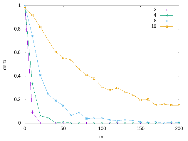
Now that we've verified our ability to find consistent hypotheses, we can answer our initial question. We can just plug the value for \(| \mathcal{H} |\) into our bound to get the solution. Since there are \(k\) literals, and we have three different options for each literal, we can say

So in this case, m is \(O(\log | \mathcal{H} |) = O(k)\) where k is the number of literals.

The whole point of this installment was to walk through the basics of PAC learning and give a few examples to help build some intuition. The main thing I hoped to emphasize was the ability of using PAC bounds to help think about the fundamentals limits of learning, and how we can use these bounds to understand what goes into problem difficulty in an empirical way. If you found these ideas interesting, I highly recommend looking into the resources I referenced in the beginning, along with An Introduction to Computational Learning Theory.